

Data Visualizations – Oceans
These animations are offered as examples of scientific research results, to convey complex information in graphic form. See also: Ocean Modeling
Redistribution of these materials is permitted, but we ask that NOAA/GFDL be credited as the source, and that we be informed of the usage. Please also see our Disclaimers and Privacy Policy. You can also create visualizations with some of GFDL’s climate data using NOAA’s data exploration tool, NOAAView.
For questions, please contact oar.gfdl.communications@noaa.gov
Large Scale Ocean Dynamics
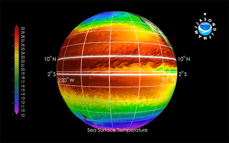
El Niño Simulation with NOAA/GFDL’s CM2.6 High Resolution Coupled Climate Model
This animation of model output illustrates the three dimensional complexity which is resolved in this model. A section of the Equatorial Pacific is showcased as it evolves through several ENSO events.
Details
Title |
El Nino Simulation with NOAA/GFDL’s CM2.6 High Resolution Coupled Climate Model. (Presented at the 20th United Nations Conference of The Parties at Lima, Peru in December 2014.) |
Description |
This animation of model output illustrates the three dimensional complexity which is resolved in this model. A section of the Equatorial Pacific is showcased as it evolves through several ENSO events. Sea surface temperatures are taken from NOAA/GFDL’s CM2.6 High Resolution Coupled Climate Model which has a nominal resolution of 1/2 degree for the land and atmosphere and 1/10 degree for the ocean and ice. The surface temperature are daily output while the subsurface temperatures are interpolated from monthly output. Salient features are the tropical instability waves and their subsurface impact, the evolution of the tropical thermocline through the events and the impacts of the presence of a well represented Galapagos Archipelago. |
Model name |
NOAA/GFDL’s CM2.6 High Resolution Coupled Climate Model |
Scientist(s) |
Whit Anderson, Tom Delworth, Tony Rosati, Mike Winton |
Date Created |
November 2014 |
Visualization personnel |
Whit Anderson, Youngrak Cho |
Files |
MPEG 1080p |
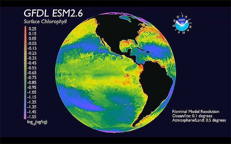
Surface Chlorophyll from NOAA/GFDL’s ESM2.6 High Resolution Earth System Model
Daily model output of surface chlorophyll is animated and shown globally. This animation highlights the models ability to simulate a biological quantity which has global ramifications on the physical and biological climate systems.
Details
Title |
Surface Chlorophyll from NOAA/GFDL’s ESM2.6 High Resolution Earth System Model. (Presented at the 20th United Nations Conference of The Parties at Lima, Peru in December 2014.) |
Description |
This animation illustrates the hourly outgoing longwave radiation (OLR) field from the global 3-km FV3 (Finite Volume Cubed-Sphere Dynamical Core). Daily model output of surface chlorophyll is animated and shown globally. This animation highlights the models ability to simulate a biological quantity which has global ramifications on the physical and biological climate systems. The model from which the chlorophyll is taken is the biogeochemically comprehensive Carbon, Ocean Biogeochemistry And Lower Trophics (COBALT). This model focuses on multi-elemental biogeochemical coupling while sacrificing ecological comprehensiveness through a high degree of ecological empirical parametrization via Dunne et al. (2005). The physical model used to drive COBALT in this simulation is NOAA/GFDL’s CM2.6 High Resolution Coupled Climate Model. |
Model name |
CM2.6 High Resolution Coupled Climate Model/COBALT |
Scientist(s) |
Whit Anderson, John Dunne, Charlie Stock, Jasmin John |
Date Created |
August 2014 |
Visualization personnel |
Whit Anderson, Youngrak Cho |
Files |
MPEG |
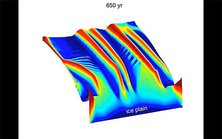
Formation of melt channels on the base of the ice shelf. Shape shows the shape of the ice-shelf base, colors show the plume flux. View from the grounding line towards ice front.
The movie shows results of simulations of a fully coupled ice-shelf-flow/sub-ice-shelf ocean circulation model. The ice shelf has no-slip conditions at the lateral boundaries. Frames are taken every 10 years.
Details
Title |
Formation of melt channels on the base of the ice shelf. Shape shows the shape of the ice-shelf base, colors show the plume flux. View from the grounding line towards ice front. |
Description |
The movie shows results of simulations of a fully coupled ice-shelf-flow/sub-ice-shelf ocean circulation model. The ice shelf has no-slip conditions at the lateral boundaries. Frames are taken every 10 years. |
Model name |
GFDL ice-shelf/sub-ice-shelf circulation model |
Scientist(s) |
Olga Sergienko |
Date Created |
November 28, 2012 |
Visualization personnel |
Olga Sergienko |
Files |
MOV (6MB) |
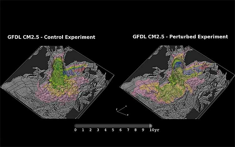
The Impact of the Nordic Sea Overflow on Passive Tracers in the North Atlantic
In the control experiment using CM2.5, the Nordic Sea overflow entered into the North Atlantic deep ocean is very weak. The passive dye is released continuously from the Denmark Strait with a constant co…
Details
Title |
The Impact of the Nordic Sea Overflow on Passive Tracers in the North Atlantic |
Description |
In the control experiment using CM2.5, the Nordic Sea overflow entered into the North Atlantic deep ocean is very weak. The passive dye is released continuously from the Denmark Strait with a constant concentration of 1. Due to the lack of a strong deep current near the western boundary south of the Flemish Cap, the younger age tracer and the passive dye released from the Denmark Strait are mainly confined to the subpolar region and do not penetrate to south of the Grand Banks. On the contrary, in the perturbed experiment, when a much stronger Nordic Sea overflow enters into the North Atlantic deep ocean through the Denmark Strait, the younger age tracer and the passive dye released from the Denmark Strait show much higher concentration near the western boundary and less eastward distribution in the interior ocean, and can reach the western North Atlantic basin south of the Grand Banks due to the advection by the stronger deep current. |
Model name |
CM2.5 |
Scientist(s) |
Alistair Adcroft, Robert Hallberg |
Date Created |
January, 2011 |
Visualization personnel |
Simon Su |
Files |
MOV (44MB) |
Gulf of Mexico Oil Spill
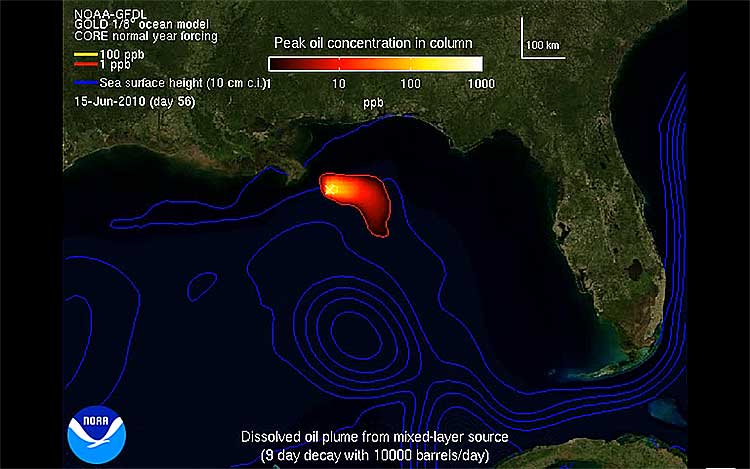
Dissolved oil plume from mixed layer source (decaying)
The simulated concentration (in parts per billion) of dissolved oil in the ocean mixed layer (near the sea surface). The simulated ocean currents used here are plausible but should not agree in detail with the observed currents.
Details
Title |
Dissolved oil plume from mixed layer source (decaying) |
Description |
The simulated concentration (in parts per billion) of dissolved oil in the ocean mixed layer (near the sea surface). The simulated ocean currents used here are plausible but should not agree in detail with the observed currents. The source of oil is steady between April 20th and July 15th but the plume wavers back and forth with the changing ocean currents. The initial position of the loop current can affect the exact location of the dissolved oil plumes, but will not substantially alter the confinement of the significant concentrations to the Northern Gulf of Mexico, provided that the microbial oxidation is taken into account. |
Model name |
|
Scientist(s) |
Alistair Adcroft, Robert Hallberg |
Date Created |
August 20, 2010 |
Visualization personnel |
|
Files |
MPG (3MB) |
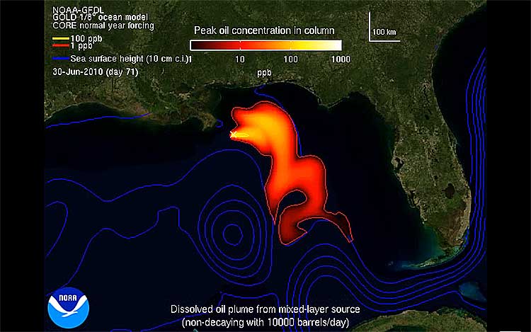
Dissolved oil plume from mixed layer source (non-decaying)
In contrast to the first animation, animation 2 shows what happens if microbial decay is omitted (as in some previous studies); the strong surface currents can spread the plume of dissolved oil throughout the Gulf of Mexico and as far as the Florida Straits and beyond.
Details
Title |
Dissolved oil plume from mixed layer source (non-decaying) |
Description |
In contrast to the first animation, animation 2 shows what happens if microbial decay is omitted (as in some previous studies); the strong surface currents can spread the plume of dissolved oil throughout the Gulf of Mexico and as far as the Florida Straits and beyond. This extensive spreading of dissolved oil is not what has been observed and we do not believe that this animation is representative of actual events. |
Model name |
|
Scientist(s) |
Alistair Adcroft, Robert Hallberg |
Date Created |
August 20, 2010 |
Visualization personnel |
|
Files |
MPG (11MB) |
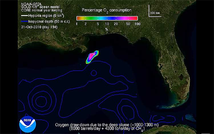
Oxygen draw-down due to the deep plume
The percentage draw down of dissolved oxygen for a 300 m thick deep plume (as a percentage of climatological levels at 1,000-1,300 m depth).
Details
Title |
Oxygen draw-down due to the deep plume |
Description |
The percentage draw down of dissolved oxygen for a 300 m thick deep plume (as a percentage of climatological levels at 1,000-1,300 m depth). The regions of significant oxygen depletion remain confined to the source region. If the actual plume were much thicker, both the hydrocarbon concentration and oxygen draw down would be proportionately smaller due to dilution. |
Model name |
|
Scientist(s) |
Alistair Adcroft, Robert Hallberg |
Date Created |
August 20, 2010 |
Visualization personnel |
|
Files |
MPG |
Ocean Temperature
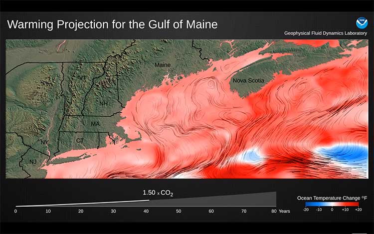
Warming Projection for the Gulf of Maine
Monthly ocean temperature and ocean current speed/direction (0-200 m) under a transient climate response (1% per year increase in atmospheric CO2).
Details
Title |
Warming Projection for the Gulf of Maine |
Description |
Monthly ocean temperature and ocean current speed/direction (0-200 m) under a transient climate response (1% per year increase in atmospheric CO2) |
Model name |
GFDL CM2.6 |
Scientist(s) |
Vincent Saba |
Date Created |
February 2016 |
Visualization personnel |
Remik Ziemlinksi |
Files |
MP4 |
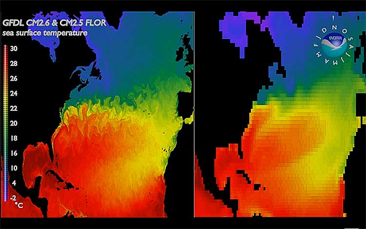
The animation shows the impact of ocean resolution on the simulation of ocean currents and eddies.
Details
Title |
Sea surface temperature simulation from 1/10o and 1o resolution ocean models coupled to the same 1/2o resolution atmosphere model. |
Description |
The animation shows the impact of ocean resolution on the simulation of ocean currents and eddies. |
Model name |
CM2.6 and CM2.5FLOR |
Scientist(s) |
Whit Anderson, Stephen Griffies, Michael Winton |
Date Created |
March 7, 2014 |
Visualization personnel |
Whit Anderson |
Files |
MOV (68MB) |
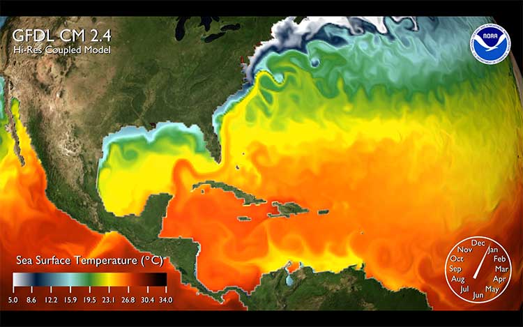
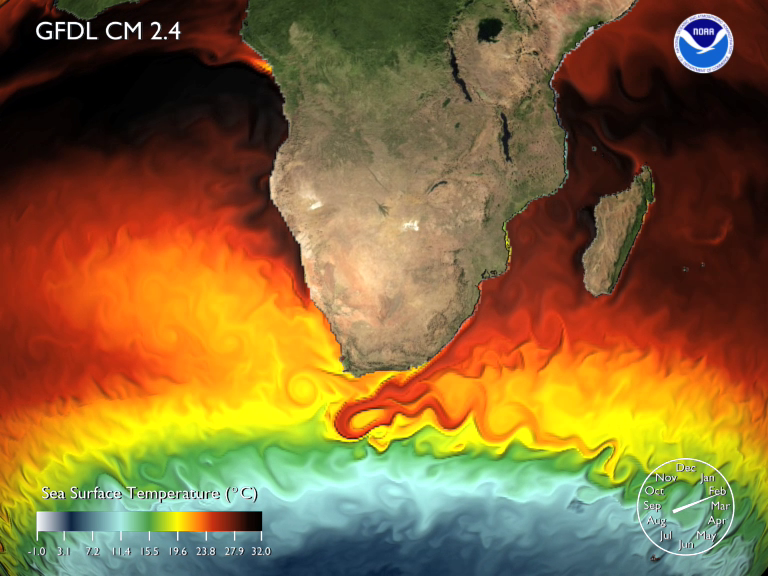
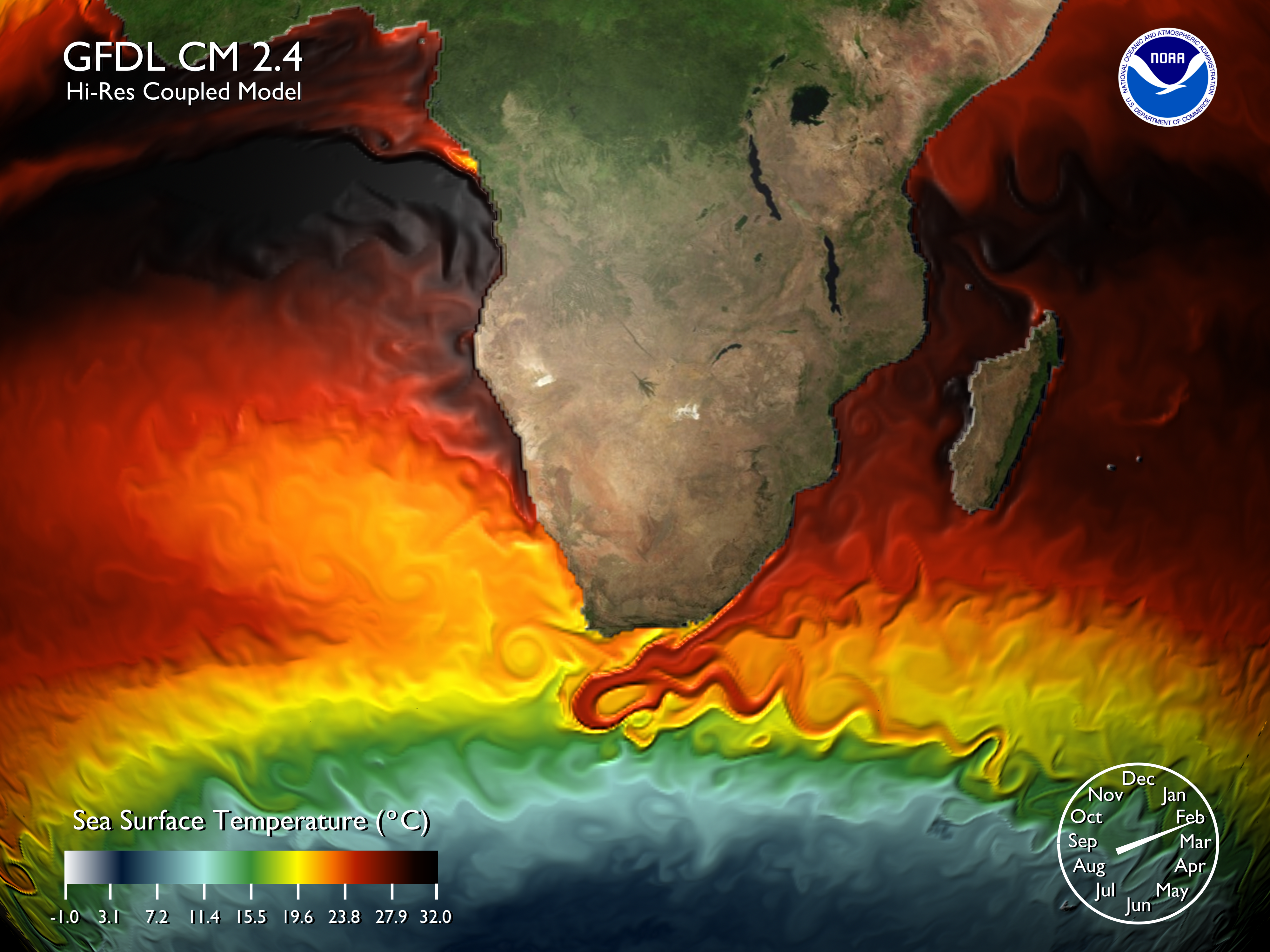
Surface Speed
Sea surface temperature (SST) simulation from GFDL’s high resolution coupled atmosphere-ocean model. As the animation focuses on various locations of the world ocean we see the major current systems…
Details
Title |
Surface Speed |
Description |
Sea surface temperature (SST) simulation from GFDL’s high resolution coupled atmosphere-ocean model. As the animation focuses on various locations of the world ocean we see the major current systems eg. the Agulhas current, Brazil current, Gulf Stream, Pacific Equatorial current, Kuroshio current. The small scale eddy structure is resolved and evident. |
Model name |
CM2.4 |
Scientist(s) |
Thomas Delworth, Anthony Rosati |
Date Created |
March 2008 |
Visualization personnel |
|
Files |
1080p High-Def Avi (56MB) 1080p High-Def Mpeg (123MB) 1080p Lossless Mpeg (3.4GB) Png (768px×576px) (1.3MB) Png (4000px×3000px) (10.8MB) Mov (116MB) Mpg (61MB) Indian Ocean Mov (67MB) Indian Ocean Wmv (72MB) |
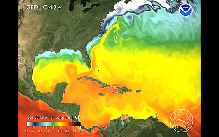
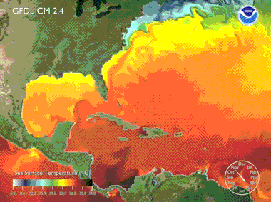
The Loop Current and the Gulf Stream
This is a simulation of the Arctic Ocean Surface Salinity from GFDL’s high resolution coupled model. One can see the seasonal cycle of summertime freshening from sea ice melt as well as the salty water entering from the North Atlantic current.
Details
Title |
The Loop Current and the Gulf Stream |
Description |
The animation focuses on the Loop Current as it flows into the Gulf Stream (a major surface current). Note the black colors indicate the warmest ocean surface temperatures and and light blues indicate the coolest temperatures. Sea surface temperature (SST) simulation from the Geophysical Fluid Dynamics Laboratory’s (GFDL) high resolution coupled atmosphere-ocean model. |
Model name |
CM2.4 |
Scientist(s) |
Anthony Rosati, Thomas Delworth |
Date Created |
|
Visualization personnel |
Remik Ziemlinksi |
Files |
MP4 (65MB) Animated GIF |
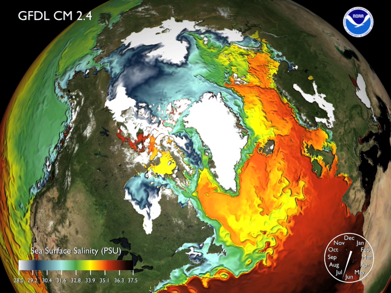
Ocean Surface Salinity
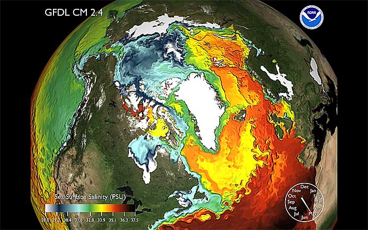
Surface Salinity
This is a simulation of the Arctic Ocean Surface Salinity from GFDL’s high resolution coupled model. One can see the seasonal cycle of summertime freshening from sea ice melt as well as the salty water entering from the North Atlantic current.
Details
Title |
Surface Salinity |
Description |
This is a simulation of the Arctic Ocean Surface Salinity from GFDL’s high resolution coupled model. One can see the seasonal cycle of summertime freshening from sea ice melt as well as the salty water entering from the North Atlantic current. |
Model name |
CM2.4 |
Scientist(s) |
Thomas Delworth, Anthony Rosati |
Date Created |
March 2008 |
Visualization personnel |
Xi Chen |
Files |
Png (1.3MB) Mov (44MB) Mpg (30MB) Indian Ocean Mov (45MB) Indian Ocean Wmv (56MB) |
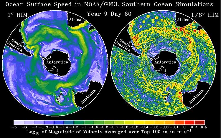
Ocean Surface Speed
Surface Speed
A three-dimensional ocean circulation model has been used for studying both the ocean climate system and more idealized ocean circulations.
Details
Title |
Surface speed |
Description |
A three-dimensional ocean circulation model has been used for studying both the ocean climate system and more idealized ocean circulations. |
Model name |
Hybrid Isopycnal Model |
Scientist(s) |
R. Hallberg |
Date Created |
|
Visualization personnel |
|
Files |
MPEG Video (19MB) |
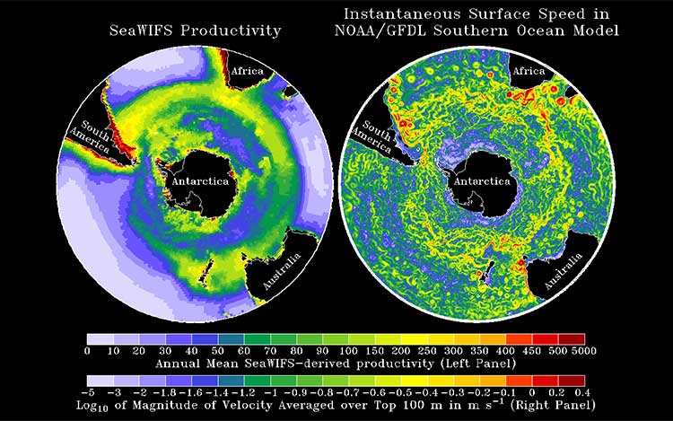
SeaWIFS Productivity vs. Surface Speed
The figure shows us that southern ocean productivity may be linked with eddy activity.
Details
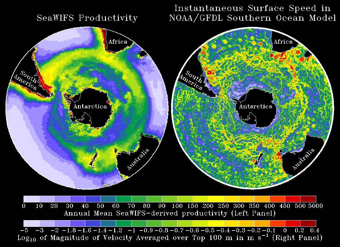
Title |
SeaWIFS Productivity vs. Surface Speed |
Description |
The figure shows us that southern ocean productivity may be linked with eddy activity. |
Model name |
Hybrid Isopycnal Model |
Scientist(s) |
R. Hallberg |
Date Created |
|
Visualization personnel |
|
Files |
PNG |