26. Relative humidity in “cloud resolving” models

Posted on April 9th, 2012 in Isaac Held's Blog

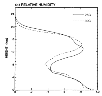
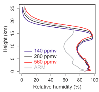
Time and spatially averaged relative humidity profiles from radiative-convective equilibrium simulations with cloud-resolving models.  The figure on the left is from Held et al, 1993 and shows results from two simulations differing by 5C  in the prescribed surface temperature. That on the right is from Romps 2011 and shows the result of changing the CO₂ and adjusting surface temperatures to keep the net flux at the top of the atmosphere unchanged.  (Also shown on the right is the observed profile at a tropical western Pacific ARM site.)

Regarding water vapor or, equivalently, relative humidity feedback, we can think of theory/modeling as providing a “prior” which is then modified by observations (trends, interannual variability, Pinatubo response). My personal “prior” is that relative humidity feedback is weak. or, conversely, that the strength of water vapor feedback in our global models is about right.

In justifying this prior, I like to start with the rather trivial argument, already mentioned in the last post, that the amount of water vapor in the atmosphere cannot possibly stay unchanged as the climate cools since many regions will become supersaturated, including the upper tropical troposphere where most of the water vapor feedback is generated..  So to expect specific humidity to remain unchanged as the climate warms requires the present climate to be close to a distinguished point as a function of temperature  – the point at which water vapor stops increasing as temperatures increase.  Its not impossible that we do reside at such a point, but you’re going to have work pretty hard to convince me of that — it doesn’t strike me as a plausible starting point.

Of course, there is also the community’s collective experience with global atmospheric models over the past several decades.  Less familiarly, there is experience more recently with the kind of “cloud-resolving” models (CRMs) discussed in Posts #19-20. I am going to focus on the latter here. This will have the advantage of introducing what I consider to be the physical mechanism that could most plausibly alter the strength of water vapor feedback.

In global climate models in use for climate studies, which typically have horizontal resolutions of 50-200 kms, most of the turbulent motions transporting heat, momentum and water vertically in the tropics are not resolved by the grid and must be provided by a sub-grid closure scheme. Our ability to develop convincing closures for moist convective turbulence remains limited. In contrast, in CRMs the horizontal grid size might be 1-3 kms, which begins to resolve the most energetic motions responsible for vertical mixing in the tropics, the convective plumes that reach from the surface to the upper troposphere. There is still sensitivity to the treatment of subgrid motions at even smaller spatial scales, but there is little doubt that the explicitly resolved deep convective plumes provide more realistic simulations of tropical mixing than our attempts at subgrid closure in global models.

One goal of this work is to devise CRM computations in small domains that provide insights into climate sensitivity. A basic starting point is radiative–convective equilibrium in a doubly periodic and, therefore, horizontally homogeneous, box. Fix the surface temperature, let the radiative fluxes cool the troposphere, and see how the convection, clouds and relative humidity distributions develop as the system achieves it statistically steady state (its climate).  Then increase the surface temperature and study how the model climate responds. (Or increase the CO₂ and iterate the surface temperature so as not to perturb the net energy flux at the top-of-atmosphere.)  I like to think of radiative-convective equilibrium as the Rayleigh-Benard Convection of climate theory.  (Unfortunately, there is no good way of simulating it in the laboratory.)

The figure on the left at the top is from one of the first CRM studies of moist radiative-convective equilibrium, with a 2D model and with the relatively low resolution of 5km. It shows the equilibrated horizontally and time averaged relative humidity profile for a control simulation and for another simulation with an increase of 5K in the imposed surface temperature.  On the upper right is the result of a more recent and much higher resolution 3D simulation.  (Here the perturbation runs have both increased surface temperature and increased CO₂, so they include what in previous posts I have called the “ultra-fast” response to CO_2, as well as the usual effects of the increase in surface temperature due to the CO₂ increase.)

The first thing to notice is that the changes in the relative humidity profile in these models as the climate warms are small. (Some aspects of these small changes, especially the upward displacement of the relative humidity profile in the upper troposphere, are robust features across simulations of this type.) The point of comparison is the reduction in relative humidity needed to maintain constant specific humidity, which would be about 6%/degree C warming near the surface to 12%/C or so in the upper troposphere. The temperature changes in these simulations are close to moist adiabatic, as shown in Post #20 for the Romps simulation. So the relative humidity feedback in these models is very weak, just as in global models. There are a lot of these cloud resolving models in the literature, in domains with different sizes and shapes, some in the “pure” radiative-convective configuration I am focusing on here, others with some specified large-scale flows superposed — they all look similar in this regard.

Something else you have probably noticed is that the relative humidities in these two models are quite different (the model on the left is drier throughout most of the troposphere). While I am only showing two models, this large spread is also representative of models of this type. The following picture is the one that I think of when looking at results such as these.

Air is carried up to the upper troposphere in deep convective plumes that extend to various heights – when the air emerges from these plumes it descends very slowly. This skewness of vertical motion, rapid ascent and slow descent, is consistent with the small areas covered by the convective plumes, and is a distinctive feature of the tropical atmosphere, as understood by Riehl and Malkus in the late 1950’s . We can think of the air as saturated when it emerges from the convective plumes, and as it descends it warms and its relative humidity quickly starts dropping. If it makes it into the lower troposphere without incident its relative humidity would be a few percent or lower!  But this decent might take 2 or 3 weeks, so descending parcels will typically mix with air that has recently been moistened by water detrained from convection at these lower levels. Near the surface the air is moistened by mixing with the water that is constantly evaporating from the oceans (these models typically assume a saturated surface), so we end up with a minimum of relative humidity in the interior of the troposphere. But the strength of this minimum depends on how far typical parcels descend before being moistened, and this depends on how the convection is organized.

Picture someone in the tropics with a big garden hose pointing upward, trying to moisten the air before it descends too far and its relative humidity drops to near zero. Standing in one place would be very ineffective –assuming that there is relatively little horizontal mixing going on — the hose would always be moistening the same small fraction of parcels, wasting water by moistening parcels that are already moist,  and allowing the troposphere as a whole to dry.  Moving the hose around or using many small hoses simultaneously so to moisten more air parcels, while using the same amount of water, would be much more effective.

Post #19 shows an example of how the organization of convection can change drastically in a CRM as a function of a model parameter.  The mid-tropospheric minimum in time-averaged relative humidity in the  aggregated state is 15% in the model described there, as constrasted with about 60% in the more disaggregated state!  CRMs differ in their mean relative humidity profiles because they organize convection differently, due to model differences of various kinds, including domain size and shape, resolution, cloud-radiation interactions, surface flux formulations, etc —  these dependencies are not well understood. Relative humidity changes are small when these models are warmed because this organization does not change significantly in response to the warming.

Could it be that convection aggregates more as the climate warms?  If you are looking for a way to weaken water vapor feedback, this is one of the better places to look., but you’ll need a lot of aggregation to compete with Clausius-Clapeyron.  Google “convective organization and water vapor feedback” to get a feel for what people are thinking about.  Are horizontally homogeneous models of radiative-convective equilibrium the appropriate theoretical tools for studying this? The problem is that they are missing a lot of the processes that generate flows that mix water vapor horizontally, mixing that likely reduces the sensitivity of humidity to convective organization. These flows are better represented in global models, despite limitations in their representations of moist convection.  CRMs in small domains may distort the big picture

Despite these possibilities, integrations with CRMs to date, such as those shown at the top, have helped solidify my theoretically-based prior, which I think of as the most conservative possible:  nothing much changes, including the convective organization.  I’ll cover the way in which observations reinforce or modify this prior eventually.

(Added on April 11)

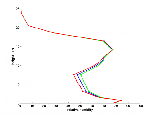
I thought I would add a plot of the time mean relative humidity simulated by the 50km global atmospheric model that I have been using for illustrative purposes in a lot of these posts — at the same geographical location (Nauru Island) for which the observed profile was included in the plot on the top-right.

The red line, the driest profile shown,  is the closest grid point to Nauru.  I then plotted several other points moving westward a total of about 10 degrees longitude.  There is an east-west gradient in humidity, with humidity increasing westward — the model’s isolines of midtropospheric humidity are displaced about 10 degrees to the west compared to observations along the equator in the western Pacific. The mid-tropospheric minimum also appears to be reached somewhat lower in the atmosphere than observed. (This is, once again, a free-running model except for the prescribed sea surface temperatures).

These GCMs and cloud-resolving models are complementary tools — we can even try to combine them in “super-parametrized” models, such as Khairoutdinov et al 2007.

[The views expressed on this blog are in no sense official positions of the Geophysical Fluid Dynamics Laboratory, the National Oceanic and Atmospheric Administration, or the Department of Commerce.]