34. Summer temperature trends over Asia

Posted on December 31st, 2012 in Isaac Held's Blog

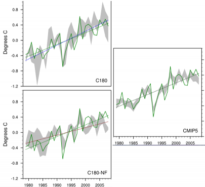
Anomalies in near surface air temperature over land (1979-2008) averaged over Asia and the months of June-July-August from CRUTEM4 (green) — and as simulated by atmosphere/land models in which oceanic boundary conditions are prescribed to follow observations (gray shading). See text and Post #32 for details.

This is a follow up to Post #32 on Northern Hemisphere land temperatures as simulated in models in which sea surface temperatures (SSTs) and sea ice extent are prescribed to follow observations.  I am interested in whether we can use simulations of this “AMIP” type to learn something about how well a climate model is handling the response of land temperatures to different forcing agents such as aerosols and well-mixed greenhouse gases.  If a model forced with prescribed SST/ice boundary conditions and prescribed variations in the forcing agents does a reasonably good job of simulating observations, we can then ask how much of this response is due to the SST variations and how much is due to the forcing agents (assuming linearity).  If the response to SST variations is robust enough, we have a chance to subtract it off and see if different assumptions about aerosol forcing, in particular, improve or degrade the fit to observations.

In post #32, the focus was on the annual mean land temperatures averaged over the Northern Hemisphere.  If you look at the model simulations in different seasons, in this prescribed SST/ice context, you see a lot more variation from realization to realization in winter than in summer due to internal atmospheric variability.  If we are interested in confronting models with the observed spatial structure of trends over land, it helps to look at the system in such a way as to minimize the influence of internal variability.  Focusing on summer is one way to get started. The idea to focus on Asia in addition is partially to try to maximize the influence of the forcing agents as opposed to the SST influence, but our AMIP simulations suggest that the spatial structure of the summertime trends is also less noisy over Asia than over N. America.  There are more systematic ways of doing this, needless to say, but I think looking at Asia in summer might be a good way to get a feeling for whether this is worth pursuing.

The figure at the top of this post shows the spatial mean of 2m land temperatures in June-July-August over Asia (35E-170W, 7N-83N) from CRUTEM4 in green. As in #32, the AMIP simulations from 17 models  in the CMIP5 archive are first averaged over all available realizations for each model, and anomalies are computed from the mean over the 1979-2008 period.  The shading in the figure on the right shows the 25%-75% range of this ensemble of model anomalies.

The figure on the upper left shows the result from one of our atmosphere/land models, HiRAM C180.  To confuse matters the shading here indicates the spread among three realizations,  a measure of internal variability.    The figure on the lower left is generated with the same model but including only SST and ice extent variations, holding the forcing agents fixed.

The temperature trends in the CMIP5 ensemble are very close to the observational estimate, while the C180 model’s trend (upper left) is a bit high — one anomalously cold season,  in ’83 near the start of this time series, seems to be partly to blame.  With forcing variations removed (lower left), the C180 model trend is reduced by more than 40%.

It is nice to see the cooling due to Pinatubo appear so clearly in the summer of ’92 (the eruption was in June ’91).  It is well simulated by the models without any additional smoothing or removal of ENSO effects. Of course, some of this is coming from the observed SST response, which is imposed here.  From the “attribution” implied by the figures on the left above, it seems that about 1/2 to 2/3 of the cooling over Asia in the summer of ’92 is communicated from the ocean, the rest coming directly from the volcanic forcing.

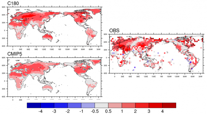
Putting the summertime trends over Asia in a global context, here is the observed spatial pattern of 30 year June-July-Aug trends as well as the results from the mean of the CMIP5 ensemble and the mean of our 3 C180 realizations.

The numbers on the color scale are in degrees C/30 yrs.  In the OBS=CRUTEM4 plot, white means that we felt that too much data was missing to compute a trend; gray, as in the other plots, means that the absolute value of the trend is less than 0.5C/30yrs.  The relatively small summer trends in this 30 year period in the eastern half of the US and in a curious slash through central Asia are some of the interesting discrepancies between these observational estimates and the mean of these model ensembles.

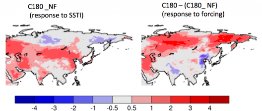
Decomposing the C180 model result over Asia into a part due to the SSTs and sea ice alone and the remainder, which we interpret as due to varying forcing agents, we get this:

I have focused this plot on Asia because that seems to be where the model decomposition is particularly robust across the different realizations.  (The analogous figure over N. America seems to be more strongly distorted by sampling of internal atmospheric variability.)  We need more realizations to look at this decomposition carefully across the globe and to test the assumption of linear superposition.  It is interesting that the response to SSTs and sea ice extent has weak cooling in Northern Asia.  Over the Arctic in summer near surface temperatures are tightly constrained to be close to the melting temperature of sea ice, so to the extent that diffusion from the Arctic is relevant this would tend to minimize the warming in adjacent land, but this mechanism would not produce cooling. Cooling is most likely related to moistening of the soil, perhaps due to increase in Spring snowfall or summer rains.  To what extent is this pattern robust across models?  (A number of other modeling centers have simulations relevant for this kind of decomposition but they are not in the CMIP5 archive.)

The remainder (on the right in the figure), which we interpret as due to forcing variations, is also interesting. The cooling or lack of warming over the southern half of the continent is presumably due in large part to aerosols.  I don’t think Pinatubo torques the trend very much since it occurs close to the middle of this time period, but that needs to be checked. There does seem to be some potential for constraining aspects of the anthropogenic aerosol forcing with this approach.

Aerosols have not been a focus of the model development leading to this HiRAM model series  (these models include the same prescribed aerosol distributions as in our earlier AM2/CM2 model series and include no indirect effects due to aerosol-cloud interactions).  In these models we have focused instead on moving to higher resolution and simulating tropical storms statistics.  Our lab’s aerosol and atmospheric chemistry modeling research has instead been directed towards our AM3/CM3 branch of models, which is driven by emissions rather than prescribed concentration fields.  We are just getting started on a development path designed in part to combine the best aspects of HiRAM and AM3 so that, among other things, we can study the influence of aerosols (including Saharan dust) on tropical storms.  A quick inspection of AM3 AMIP simulations suggests a decomposition between forcing and SST components different from that described above. (Thanks to Yi Ming for a look at the AM3 results and to Bruce Wyman for generating the figures in this post.)

[The views expressed on this blog are in no sense official positions of the Geophysical Fluid Dynamics Laboratory, the National Oceanic and Atmospheric Administration, or the Department of Commerce.]