73. Tuning to the global mean temperature record

Posted on November 28th, 2016 in Isaac Held's Blog

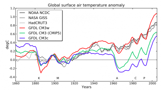
Global mean surface air temperature evolution (with 5-year running mean) in 3 versions of GFDL’s CM3 model (Donner et al, 2011), compared to observations.  Each model result is an average over 5 ensemble members. Base period is 1881-1920. From Golaz et al, 2013.

The goal of climate modeling is to develop multi-purpose climate simulators. The same model generating the global mean temperature in this figure is also used to simulate the response of tropospheric winds to the Antarctic stratospheric ozone hole, for example. But as we all know, some aspects of the simulations in our current models are robust while others are sensitive to model uncertainties and may be tunable to some extent within the context of a particular model.   If you have a simple model that you are fitting to some data, there is no problem in describing in detail how you decided on the model, the free parameters, the fitting procedure, the data used, etc. it can be more of a challenge to make the development path of a climate simulator fully transparent.

A question that gets a lot of attention is whether you should try to tune your model to be consistent with the evolution of global mean temperatures (GMT) over the past century, or if you should withhold that particular iconic data set during model development, justifying its use as a measure of model quality.

My impression is that it is the advent of models incorporating indirect aerosol effects – the effects aerosols have on climate through their modification of clouds — that has really brought this question to the forefront. The evolution of GMT is controlled by a combination of climate sensitivity, radiative forcing, and internal variability. I don’t know of any way to robustly increase or decrease a model’s internal variability on decadal and longer time scales. But in a given model you can often find ways of altering the model’s climate sensitivity through the sub-grid convection and cloud schemes that affect cloud feedback, but you have to tread carefully because the cloud simulation exerts a powerful control on the atmospheric circulation, top-of-atmosphere (TOA) and surface radiative flux patterns, the tropical precipitation distribution, etc. But including aerosol indirect effects on radiative forcing has made it easier to generate a greater variety of 20^th century simulations without affecting other aspects of the climate simulation as strongly.

The figure at the top from Golaz et al, 2013 shows simulations from three versions of the CM3 coupled atmosphere-ocean model developed at GFDL (Donner, et al 2011). This was our lab’s first attempt to incorporate the indirect effects of aerosols in a climate model. The three models are the result of varying a single parameter that controls the amount of cloud water required for the onset of coalescence in the models microphysics scheme, which in turn controls the water content of clouds. (Other parts of the model need to be adjusted to retrieve a good global mean TOA energy balance but are not the main drivers of this behavior.)

One of these versions clearly provides a better fit than the others. These differences are primarily due to aerosol radiative forcing, not climate sensitivity. The model that is most consistent with the observed evolution has the smallest aerosol forcing. (The figure shows 5-member ensemble means; individual realizations do not change the basic picture.) As described in Suzuki et al 2013, the value of the parameter that provides the best fit is not the one preferred by comparing directly to cloud observations; the settings that result in larger aerosol forcing seem more justifiable at face value. There is nothing mysterious about this. It’s an example of the familiar tension resulting from the imperfections of any model and the need to weight different performance metrics relative to each other.

So how much should we weight the importance of the simulation of the historical warming relative to other observational constraints? Personally, I think it deserves a lot of weight. I prefer if possible to study models that provide a viable hypothesis for 20^th century temperature change, pushing against other observational constraints as a necessary expedient. You might be able to arrange climate modelers along an expediency spectrum depending on how they weight low level constraints vis-a-vis more holistic aspects of the climate simulation.

In general, the quality of the 20th century trend has to be considered somehow along with other metrics deemed to be of significance. How much weight would need to be placed on these trends to say that they were “tuned”? Imagine a best case scenario in which weights are made explicit and the optimization is performed by an explicit algorithm. You would presumably have to give up on binary tuned/no tuned categories and know a lot of details about the optimization procedure if you really cared to quantify this. But this best case scenario is rarely relevant — why this is so is an interesting question that could be the topic of another post.

“Tuning” to the 20^th century temperature trends is itself ambiguous. In particular, initial stages of atmospheric model development often take place without coupling to an ocean model, running instead over observed sea surface temperatures (SSTs) and sea ice extent. It is fairly standard to compute the Cess sensitivity (CS), increasing SSTs uniformly by some amount, 2K is common, and looking at the increase in the net radiation at the TOA, per degree. This computation gives you a first inkling of the model’s climate sensitivity. Another standard computation is to hold the SSTs and sea ice fixed and change all radiative forcing agents from present day to pre-industrial values. Looking again at the change in the TOA energy balance, we call this change the effective radiative forcing or radiative flux perturbation RFP. Dividing RFP by CS gives you a scale for the temperature change from pre-industrial to the present day. It’s not quantitative for several reasons (ocean heat uptake, the dependence of radiative feedbacks on the spatial structure of the SST changes, etc). But it is a reasonable expectation (whether it is always true is a separate question) that if you make a change in the atmospheric model that affects RFP/CS substantially, your overall warming from pre-industrial-to-present in the fully coupled model will change in the same direction. Suppose a modeling group is doing this routinely and sees that a proposed change in the model atmosphere modifies RFP/CS in a way that would likely push a coupled model in the wrong direction — and as a result this change is not accepted. Is this “tuning” to past GMT evolution, even though the model has not actually been used to simulate this evolution explicitly?

You could go further and talk about tuning to “emergent constraints” for climate sensitivity, observational metrics that are correlated with climate sensitivity when looking across model ensembles. Is it “tuning” of the 20^th century temperature record if your decisions are justified on the basis of these emergent constraints alone and not the GMT evolution with a fully coupled model? Your answer might depend on whether you find this literature on emergent constraints convincing or not.

But irrespective of all these details, the key point, I think, is that bottom-up, first principles modeling coupled with observational constraints other than the observed GMT evolution still leave room to generate a substantial spread in aerosol forcing and climate sensitivity. So what does it mean if a group manages to get a good simulation without tuning? Were they lucky? Have they made a case for reduced uncertainty? Is being satisfied with a first attempt and not exploring the consequences of this uncertainty a form of implicit tuning?

I was interviewed recently for a news article on climate model tuning, which said: … nearly every model has been calibrated precisely to the 20th century climate records—otherwise it would have ended up in the trash. “It’s fair to say all models have tuned it,” says Isaac Held . The word “precisely” changes the flavor of this sentence a lot, raising the spectre of overfitting. (I have no memory of using that word.) But I don’t doubt that I did say the part inside the quotes. I am not very good at provided sound bites. Consistent with this post, a more accurate and long-winded sound bite would have been something like — in light of the continuing uncertainty in aerosol forcing and climate sensitivity, I think it’s reasonable to assume that there has been some tuning, implicit if not explicit, in models that fit the GMT evolution well.

So is it worthwhile digging into the model development process and trying to quantify the explicit component of the tuning? I am all for transparency, and it is potentially useful as a reference to have the development path laid out in detail as best one can. But implicit tuning, which has the potential for coming into play when the target date set is as well known as the GMT evolution, is harder to quantify.  In addition, just speaking for myself (as always in this blog), life is short, and it’s not easy finding actionable intelligence in the details of a development path except where the process has clearly isolated an interesting dependency — some aspect of the simulation depending on the model formulation in an unappreciated way — in which case that dependency would probably need to be analyzed in detail in a stand-alone study that ideally made a case for robustness, without being mixed with the more contingent aspects of the model development trajectory.

Thanks to Chris Golaz, Larry Horowitz, Leo Donner, Ming Zhao, and Mike Winton for discussions on this topic.

[The views expressed on this blog are in no sense official positions of the Geophysical Fluid Dynamics Laboratory, the National Oceanic and Atmospheric Administration, or the Department of Commerce.]